Introduction

Accurate cloud cost forecasts let FinOps, engineering, and finance teams create budgets reliably, reduce surprises, and make smarter procurement decisions. This hands-on guide explains how to select models, validate accuracy, simulate scenarios, and operationalize forecasts across AWS, GCP, and Azure.

I've seen organizations cut budget variance from 40% to under 10% simply by implementing systematic forecasting. The difference isn't complex algorithms; it's having a repeatable process, clean data, and the right validation framework. Whether you're justifying a $2M Savings Plan or explaining next quarter's spike to your CFO, forecasting transforms reactive cost management into strategic planning.

Key Highlights / Takeaways

• Structured forecasting can reduce budget variance from 25 to 40 percent down to under 10 percent while improving commitment utilization by 15 to 25 percent
  
  

• Short, medium, and long term forecasts each have clear horizons, lookback windows, and target MAPE ranges that align with operational, budgeting, and strategic use cases
  
  

• Forecasting with confidence intervals enables safer commitment sizing: commit to 90% of the lower bound to capture 20-30% discounts while maintaining 85%+ utilization even in low-growth scenarios
  
  

• Clean data is non negotiable: daily CUR or billing exports, 85 to 95 percent tagging coverage, and a maintained business event calendar typically improve accuracy by 20 to 30 percent
  
  

• A simple model ladder works best in practice: moving averages for baselines, exponential smoothing for seasonality, ARIMA for intervals, and ML for complex multi feature drivers
  
  

• Native cloud forecasts from AWS, GCP, and Azure are useful for directional and executive views but are usually insufficient for commitment planning and multi cloud governance
  
  

• SaaS and advanced models earn their keep when annual cloud spend exceeds roughly 500K, multi cloud complexity increases, or accuracy needs to be better than 15 percent MAPE
  
  

• Forecasts only create value when operationalized with ownership, monthly accuracy reviews, variance analysis, and procurement workflows such as Savings Plans and RI sizing based on confidence bounds
  
  

• Systematic forecasting reduces CFO escalations and month-end fire drills by identifying variances on day 10 instead of day 28, giving teams 2-3 weeks to investigate and remediate
  
  

1. Why Forecasting Matters: Business & FinOps Outcomes

Cloud cost forecasting isn't just about predicting numbers; it's the foundation for strategic financial operations. Organizations with mature forecasting practices typically maintain budget variance under 8%, compared to 25-40% for teams relying on last month's actuals multiplied by growth assumptions.

Procurement & Commitment Planning: Here's where forecasting delivers measurable ROI. A well-calibrated forecast lets you right-size Savings Plans and Reserved Instances with confidence. For example, if your forecast shows consistent $150K/month compute spend with 95% confidence intervals of ±$12K, you can commit to $140K monthly and capture 20-30% savings without overcommitting. Teams that can't forecast usage bands accurately often leave $200K+ annually on the table.

Financial Close & Capacity Planning: Month-end close becomes predictable when finance teams can compare actuals against forecasts throughout the billing period. Rather than discovering a $50K overrun on day 28, you identify variance on day 10 and investigate

immediately. Engineering teams gain visibility into cost implications before launching new services, enabling proactive capacity provisioning rather than reactive scaling at surge pricing.

The business case is straightforward: organizations implementing structured forecasting typically see 15-25% improvement in commitment utilization, 40-60% reduction in budget variance, and 3-5 hours saved per week in variance analysis. At a broader level, cloud cost optimization is the continuous discipline of aligning cloud spend with actual business value, and accurate forecasting is what transforms that discipline from reactive cost control into proactive financial strategy.

2. Types of Forecasts & Time Horizons

Different business needs require different forecasting approaches. Matching the right horizon to your use case dramatically improves both accuracy and usefulness.

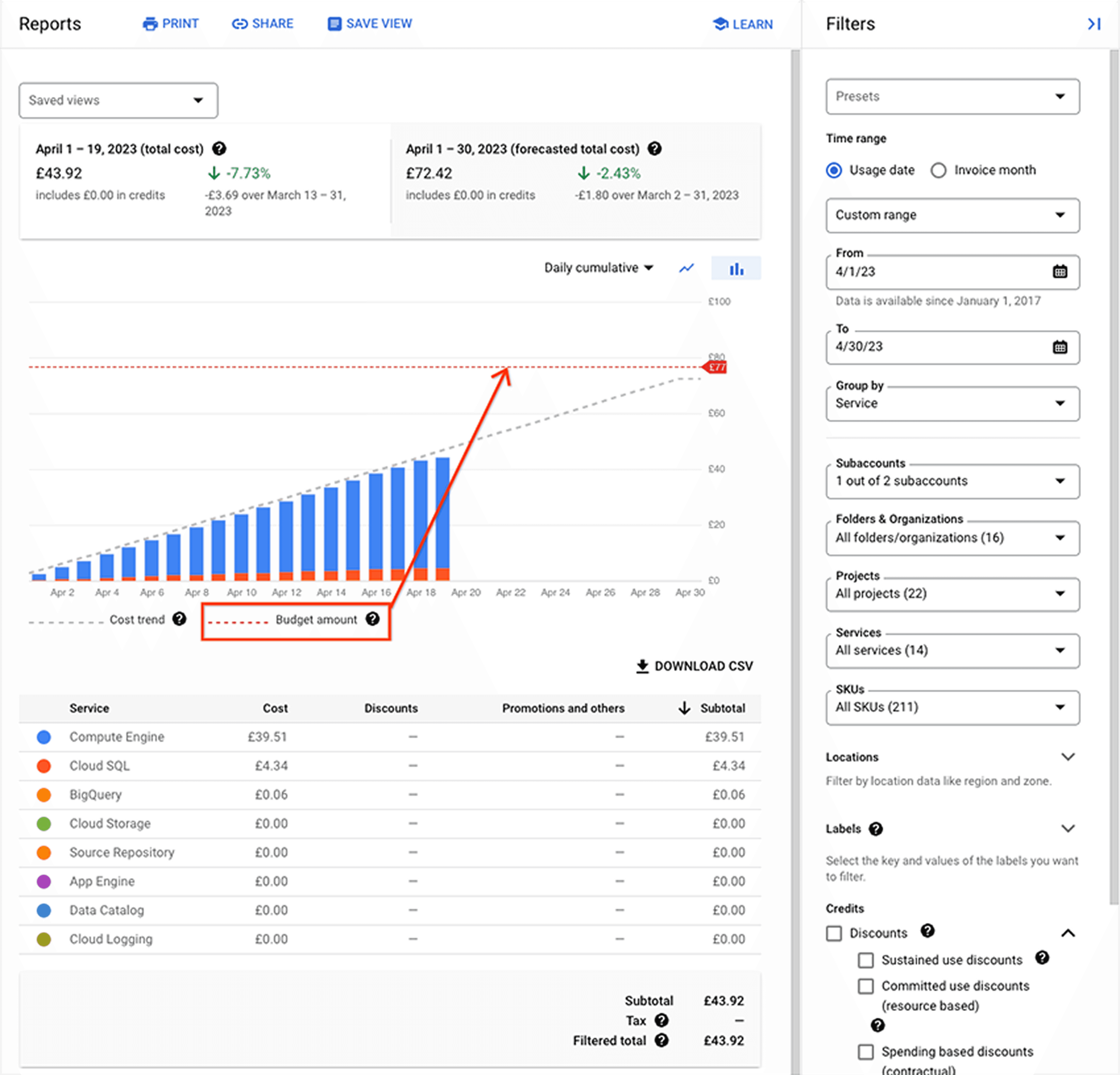
Short-Term Forecasts (1 to 3 Months): Use for monthly budgeting, variance monitoring, and operational alerting. Update weekly or daily with 60-90 days of lookback data. Target accuracy: ±5-10% MAPE for stable workloads. These forecasts catch anomalies before they compound and are essential for month-end close processes.

Medium-Term Forecasts (3 to 12 Months): Critical for annual budgeting, quarterly planning, and commitment procurement. Update monthly with 12-18 months of lookback data. Target accuracy: ±8-15% MAPE. These forecasts balance seasonal patterns with growth trends and inform Savings Plans and Reserved Instance decisions requiring 1-3 year commitments.

Long-Term Forecasts (12 to 36+ Months): Inform strategic decisions like data center exits, multi-cloud strategies, and enterprise discount negotiations. Update quarterly with 18-36 months of lookback data. Target accuracy: ±15-25% MAPE. These forecasts rely heavily on business growth assumptions and product roadmap timelines; they're less about precision and more about directional planning.

3. Data Inputs: What You Need and How to Prepare It

Forecasting accuracy lives or dies on data quality. You can have the most sophisticated model in the world, but if you're feeding it messy, incomplete, or irrelevant data, your forecasts will be garbage.

Essential Data Sources: Your primary input is historical daily cost data from AWS Cost and Usage Reports (CUR), GCP BigQuery billing exports, or Azure Cost Management APIs. Key fields include date, service, cost, usage_amount, usage_type, and resource_id.

Example:

S3 cost optimization plays a critical role in forecast accuracy because lifecycle transitions, storage class mix, retrieval behavior, and data growth rates materially change both baseline spend and future cost trajectories.

Cost Allocation Tags: Tags let you forecast at meaningful business dimensions: team, product, environment, cost center. Without proper tagging, you're forecasting the entire cloud estate as one black box. Enforce a tagging policy that includes at minimum: environment, team, application, and project. Most organizations need 85-95% tagging coverage before forecasting becomes reliable at the tag level.

Business Event Calendar: This is the secret weapon most teams overlook. Maintain a simple calendar of known events that impact usage:

Encoding these events dramatically improves forecast accuracy during non-standard periods. Without this, your model treats Black Friday as an anomaly to smooth over rather than an expected pattern.

Data Cleaning Best Practices:

• Handle missing tags by assigning to "Untagged" category and tracking coverage metrics

• Remove one-time events (large migrations, RI upfront fees, architectural refactors)

• Normalize for calendar effects; months have different lengths (28-31 days)

• Aggregate to your forecast granularity (daily data to monthly forecasts)

• Create feature variables: day of week, month of year, growth rates, commitment coverage

Clean, well-prepared data typically improves forecast accuracy by 20-30% compared to raw billing exports.

4.Models & Methods: From Simple to Advanced

Forecasting models range from basic averages to sophisticated machine learning. The right choice depends on your data characteristics, required accuracy, and operational maturity.

Moving Average: Simplest approach: average recent costs and project forward. A 30-day simple moving average predicts next month as the average of the last 30 days. Best for stable workloads and teams new to forecasting. Typical MAPE: 15-25%.

Exponential Smoothing (ETS): Applies weighted averages where recent data has exponentially higher weight. Triple Exponential Smoothing (Holt-Winters) handles level, trend, and seasonality. Best for workloads with seasonal patterns. 

Typical MAPE: 10-18%.

ARIMA: Captures autocorrelation and moving average components.  ARIMA(p,d,q) represents autoregressive order, differencing order, and moving average order. Best when you need prediction intervals and have 100+ observations.

Typical MAPE: 8-15%.

Example implementation: Statsmodels ARIMA Documentation

Machine Learning Regression: Treats forecasting as regression using historical features to predict future costs. XGBoost and Random Forest naturally handle multiple features (business events, growth metrics, resource counts). Best for complex drivers and non-linear relationships. Typical MAPE: 6-12%.

Accuracy Metrics Explained:

• MAPE (Mean Absolute Percentage Error): Most intuitive: "on average, forecasts are off by X%." Target MAPE under 15% for medium-term forecasts.

• RMSE (Root Mean Squared Error): Penalizes large errors more heavily. Useful when occasional large misses are particularly costly.

• Bias: Reveals systematic over- or under-forecasting. Zero is ideal.

When Choosing Models: Start simple (moving average) to establish a baseline. Add complexity (exponential smoothing) if you have seasonality. Move to ARIMA or ML only if simpler models don't meet accuracy targets. Always validate on held-out test data.

5.Provider-Specific How-Tos: AWS, GCP, and Azure

Each cloud provider offers native forecasting capabilities. These built-in tools are convenient for quick visibility but have limitations compared to custom models using cloud cost optimization strategies .

AWS Cost Explorer Forecasting:

1. Navigate to AWS Billing Console → Cost Explorer → Launch Cost Explorer

2. Select historical period (minimum 2 weeks, 2-3 months recommended)

3. Click "Forecast" toggle, select forecast period (1-12 months)

4. Filter by service, account, tag values

5. Download CSV with forecasted amounts and confidence intervals

Limitations: Requires 14+ days data, maximum 12-month horizon, algorithm opacity, limited seasonal handling, no custom features.

GCP Cloud Billing Forecast:

1. Navigate to Cloud Console → Billing → Reports

2. Forecast appears automatically if 30+ days billing history exists

3. Toggle forecast view, configure time range and filters

4. Export to BigQuery for programmatic access
   
   

Limitations: 30 days minimum data, maximum 3-month horizon, monthly granularity only, 4-6 hour export lag, no scenario modeling.

Azure Cost Management:

1. Navigate to Azure Portal → Cost Management + Billing → Cost analysis

2. Select scope (subscription/resource group), date range (6-12 months)

3. Toggle "Forecast" option, adjust horizon (1 to 12 months)

4. Export via Azure CLI for automation
   
   

Limitations: 10 days minimum data, 80% confidence intervals only, requires consistent tagging for tag-level forecasts.

Provider Comparison:

Use native forecasts for quick visibility and executive dashboards, but don't rely on them for procurement decisions or accuracy-critical use cases.

6. SaaS vs Native Forecasting: Comparison & Decision Framework

Native provider features and dedicated SaaS platforms together represent cloud cost optimization tools that turn raw billing data into forecasts, scenarios, and procurement decisions at scale. Choosing between native provider tools and dedicated SaaS forecasting platforms is one of the most impactful decisions for your FinOps practice.

Opsolute’s Forecast model delivers insights through predictive analysis, resource-level forecasting, budget reconciliation, and trend forecasting which helps organizations understand and interpret forecasts more accurately.

When Native Forecasting Makes Sense:

• Single-cloud organization with no multi-cloud plans

• Basic needs for directional forecasts and executive dashboards

• Budget constraints preventing SaaS investment

• Simple, stable workloads with minimal seasonality

• Early FinOps maturity, learning forecasting basics
  
  

When SaaS Platforms Are Worth It:

• Multi-cloud environment (AWS + GCP and/or Azure)

• High cloud spend ($500K+ annually) where 2-3% accuracy improvement saves $10K-$15K

• Significant commitments requiring precise usage forecasting

• Complex workloads with strong seasonality or rapid growth

• Mature FinOps practice needing automation and governance

• Budget variance must stay under 10%
  
  

ROI Example: A 500-person SaaS company spending $2.5M/year across AWS and GCP implemented a SaaS platform. It reduced MAPE from 22% to 9%, identified $120K in commitment optimization, and saved 15 hours/month in manual reconciliation. ROI: 8-10x in year one.

7.Scenario Modeling & Procurement Decisions

Forecasts become truly valuable when you use them to model "what-if" scenarios and drive procurement decisions.

Savings Plan Sizing Example: Let's work through a real-world scenario. You've forecasted EC2 compute spend at $105K/month with 95% confidence interval of $98K to $113K. Here's how to calculate your recommended commitment:

We use 90% coverage (not 100%) to avoid overcommitment risk. The remaining 10% runs on-demand, providing flexibility for unexpected spikes.

Low Growth Calculation:

• Monthly commitment: $88,200 (you pay this regardless of usage)

• Discount rate on committed amount: 22%

• Commitment cost to you: $88,200 × (1 - 0.22) = $68,796/month

• Actual spend: $95,000/month

• Remaining on-demand: $95,000 - $88,200 = $6,800/month at full price

• Total monthly cost: $68,796 + $6,800 = $75,596

• Without Savings Plan: $95,000/month

• Monthly savings: $95,000 - $75,596 = $19,404

• Annual savings: $19,404 × 12 = $232,848
  
  

High Growth Scenario Calculation:

• Monthly commitment: $88,200 (fully utilized)

• Commitment cost: $68,796/month

• Actual spend: $120,000/month

• Remaining on-demand: $120,000 - $88,200 = $31,800/month at full price

• Total monthly cost: $68,796 + $31,800 = $100,596

• Without Savings Plan: $120,000/month

• Monthly savings: $120,000 - $100,596 = $19,404

• Annual savings: $19,404 × 12 = $232,848

• Note: At this usage level, consider layering additional commitment

The math shows that even in the low-growth scenario where actual spend drops to $95K/month, you maintain 93% commitment utilization and still save $232K+ annually. This is a low-risk decision with strong downside protection.

Reserved Instance Analysis: Running 50× RDS db.r5.2xlarge instances at $1.632/hour on-demand = $714,816 annually. RI options:

• No Upfront: $471,379 annually → Save $243,437 (34%)

• Partial Upfront: $26K upfront + $410K annually = $436K → Save $279K (39%)

• All Upfront: $467K upfront → Save $247K (35%)

Partial Upfront delivers the best savings with a payback period of just over one month. The breakeven usage is 61%,  meaning that even when only 30 out of 50 instances are utilized, Reserved Instances still outperform On-Demand pricing.

Risk Containment vs Upside Capture Strategy:

When sizing commitments, balance downside protection against upside opportunity. Conservative teams commit to the 10th percentile of forecasted spend (capturing 60-70% coverage with minimal overcommitment risk), while aggressive teams commit to the 50th percentile (85-90% coverage with higher exposure to underutilization). 

The optimal approach depends on your risk tolerance and growth trajectory: stable workloads favor aggressive commitments (higher savings), while rapid-growth or volatile workloads favor conservative commitments (flexibility protection). Most mature FinOps teams target the 25th percentile (75-80% coverage), balancing $150K-$200K in annual savings against $20K-$30K in overcommitment risk for every $1M in forecasted spend.

8.Measuring Forecast Accuracy & Continuous Improvement

Metrics such as MAPE, bias, peak-to-average ratio, commitment utilization, and budget variance are core cloud cost optimization metrics because they connect forecast accuracy directly to financial outcomes and decision quality.

Track these KPIs to measure forecast quality:

MAPE (Mean Absolute Percentage Error): MAPE is the most widely used forecast accuracy metric, expressing error as a percentage of actual values. According to Wikipedia and Oracle's forecasting documentation, the formula is:

Bias: Bias reveals systematic over-forecasting (negative bias) or under-forecasting (positive bias). The formula evaluates whether forecasts consistently overestimate or underestimate demand:

Peak-to-Average Ratio: Identify volatility in spending patterns. High ratios indicate workloads with significant spikes requiring wider confidence intervals.

Accuracy Tracking Template:

Note on MAPE and Bias values in the template: The values for MAPE and Bias appear numerically identical in the single-row entries above because, for a single data point, the magnitude of the Mean Absolute Percentage Error (MAPE, which is always positive) is the same as the magnitude of the Bias Percentage (which includes a positive or negative sign). These metrics become distinct when aggregated over an entire period or multiple services, where positive and negative bias errors can offset each other.

Review accuracy monthly. If MAPE exceeds 15%, investigate root causes: architectural changes, tagging coverage drops, business events not encoded, insufficient lookback data, or model staleness.

Continuous Improvement Process:

1. Compare forecasts to actuals each month

2. Document variance drivers (planned vs unplanned)

3. Update business event calendar

4. Retrain models quarterly with fresh data

5. Adjust confidence intervals based on observed accuracy

9.Operationalizing Forecasts: Playbook & Rollout

Implementation requires clear ownership, cadence, and governance.

Ownership Model:

• FinOps Team: Owns forecast process, model maintenance, accuracy tracking

• Finance Team: Consumes forecasts for budgeting, variance analysis

• Engineering Teams: Provide input on planned changes, validate service-level forecasts

• Procurement/Contracts: Uses forecasts for commitment decisions

Cadence & Governance:

• Daily: Automated forecast refreshes for operational monitoring

• Weekly: Variance alerts when actuals deviate >15% from forecast

• Monthly: Accuracy review, forecast vs actuals reconciliation, model retraining

• Quarterly: Strategic forecast review, long-term horizon updates, commitment planning

Embedding into Monthly Close:

1. Day 1 to 5: Initial forecast vs actual comparison

2. Day 5 to 10: Investigate variances >10%, document drivers

3. Day 10 to 15: Update forecasts with actual spend, reforecast remainder of month

4. Day 15+: Final variance report to finance, root cause analysis

5. Day 25 to 30: Lock forecasts for next month, publish to stakeholders

Mid-Month vs Month-End Variance Benchmarks:

• Day 10-15: Acceptable variance ±15-20% (incomplete data, timing effects)

• Day 25-30: Target variance under ±8-10% (near-complete actuals)

• Month-End Close: Mature teams achieve ±5-7% variance consistently

If variance exceeds these thresholds, investigate immediately rather than waiting for month-end reconciliation.

Success Metrics:

• Budget variance <10% monthly

• MAPE <15% for 3-month forecasts

• Commitment utilization >85%

• Time spent on variance analysis reduced 50%

10.Common Pitfalls & Troubleshooting

Overfitting: Training models on insufficient data or too many features. Solution: Use cross-validation, start simple, add complexity only when validated.

Insufficient Lookback Data: Using <60 days for workloads with weekly seasonality. Solution: Ensure minimum 2-3 seasonal cycles in training data (8-12 weeks for weekly patterns, 18-24 months for annual).

Ignoring Business Events: Models treating Black Friday as anomaly rather than pattern. Solution: Maintain business event calendar, encode as features or manual adjustments.

Stale Models: Using 12-month-old training data for rapidly evolving architectures. Solution: Retrain monthly with rolling windows, validate accuracy regularly.

Poor Tagging Coverage: Forecasting at tag level with <80% coverage. Solution: Improve tagging before tag-level forecasting, use service-level as fallback.

Security Considerations for SaaS: When using third-party platforms, ensure read-only API access, SOC 2 Type II compliance, data encryption, and role-based access control. Never grant write permissions to billing accounts.

TL;DR + Executive Summary

Cloud cost forecasting enables accurate budgeting, optimized procurement, and proactive capacity planning. Organizations implementing systematic forecasting reduce budget variance from 25-40% to under 10% and capture 15-25% improvement in commitment utilization.

6-Point Implementation Checklist:

1. Prepare clean data: 60-90 days minimum, 85%+ tagging coverage, business event calendar

2. Select model: Start simple (exponential smoothing), add complexity only when needed

3. Validate accuracy: Test on held-out data, target MAPE <15% for medium-term forecasts

4. Track KPIs: MAPE, bias, peak-to-average ratio, review monthly

5. Operationalize: Define ownership, establish cadence, embed into monthly close

6. Optimize procurement: Use forecasts to size commitments conservatively (90% coverage of lower confidence bound)

Horizon Quick Reference:

Start with native provider tools for quick wins, graduate to custom models or SaaS platforms when accuracy requirements exceed 15% or multi-cloud support is needed. The most successful forecasting practices balance statistical rigor with operational pragmatism, perfect accuracy is impossible, but 10-15% MAPE is sufficient for most procurement and budgeting decisions.

FAQs

Q: What lookback period should I use for cloud cost forecasts?
Use 60-90 days for volatile workloads, 12 months for seasonality and budgeting, and 12-60 months for procurement planning. Always validate by testing MAPE or RMSE.

Q: How do I interpret confidence intervals?
They represent the range in which spend is expected to fall (e.g., 95% probability). Use lower bound for conservative commitment sizing and upper bound for contingency budgets.

Q: When should I use native vs SaaS forecasting?
Native = quick setup, single-cloud, directional visibility. SaaS = multi-cloud, deeper modeling, long horizon, governance, and accuracy <15% MAPE.

Q: How can I include business events or one-offs?
Maintain a business event calendar and encode it as features in ML models or manual adjustments in statistical models.

Q: What KPIs measure forecast quality?
Track MAPE, bias, RMSE, and peak-to-average ratio, visualizing drift over time in monthly accuracy reports.

Q: How do I decide on commit sizes (Savings Plans / RIs)?
Use forecasted lower confidence bound × 90% coverage target. Model downside scenarios to ensure breakeven utilization is achievable even in low-growth cases.

Q: Why might provider forecasts fail?
Common causes: insufficient history (<30 days), missing tags, data spikes, unsupported granularity, or recent architectural changes invalidating historical patterns.

Ready to improve your cloud cost forecasting? Start with clean data, simple models, and systematic accuracy tracking. With Opsolute’s intelligent forecasting framework, you can evolve from basic models to advanced techniques only when validated improvements justify the complexity. The goal isn’t perfection, it’s actionable insights that drive smarter, data-backed financial decisions.